Reading, summarizing, customizing, and plotting CDMetaPOP outputs
1 Overview
This vignette shows how to use cdmetapopR to read, reshape, summarize, and plot CDMetaPOP outputs. The goal is to show both quick plotting functions and the lower-level data-frame outputs that can be used for custom ggplot2 figures.
The examples use the package example output files in inst/extdata/Adaptive_Run_08.
1.1 Choosing Runs, Batches, Monte Carlo Replicates, and Species
Most summary functions use the same filtering arguments:
run = 0
batch = 0
mc = 0
species = 0
These defaults intentionally select one output folder. Use "all" or a range of values c(0,1) for any of these arguments to combine multiple folders. The example directory includes two batches with two MCs each. Each of these files contains ten ind#.csvs, containing information from each year of the simulation. Additionally, each file has a summary_popAllTime.csv, summary_classAllTime.csv, and a summary_popAllTime_DiseaseStates.csv that summarizes information across the years of the simulation.
one_mc <-summary_dataframe(ex_dir, type ="ind", years =9, mc =0)both_mcs <-summary_dataframe(ex_dir, type ="ind", years =9, mc ="all")all_batches_mcs <-summary_dataframe(ex_dir, type ="pop", batch ="all", mc ="all")c(one_mc_rows =nrow(one_mc),both_mcs_rows =nrow(both_mcs),all_batches_mcs_rows =nrow(all_batches_mcs))
For individual files, years narrows the selected ind##.csv files. For summary files, years are filtered after reading by using ordinary data-frame operations.
2 Conversion Helpers
2.1create_cdmat()
Use create_cdmat() to create a cost distance matrix from patch coordinates. The simplest options are Euclidean distance and equal distance.
Use cdmetapop_to_gene() to convert an ind##.csv file to GENEPOP or GENALEX format. The function writes the converted file to the current working directory, so this example uses a temporary directory.
old_wd <-getwd()setwd(tempdir())cdmetapop_to_gene(ind_file, format ="genepop")list.files(pattern ="^my_genepop")
[1] "my_genepop_ind9.txt"
setwd(old_wd)
3 Output Data Frames
summary_dataframe() returns CDMetaPOP output files as data frames for custom plotting or analysis. Use type to choose the file family and run, batch, mc, and species to choose which output folders to include. For type = "pop" and type = "class", pipe-delimited summary columns are split into one row per patch or class (depending on type) by default while keeping metrics in separate columns.
pop_df <-summary_dataframe(ex_dir, type ="pop", batch =0, mc =0)head(pop_df[, c("Year", ".batch", ".mc", "PatchID", "GrowthRate", "K", "N_Initial")])
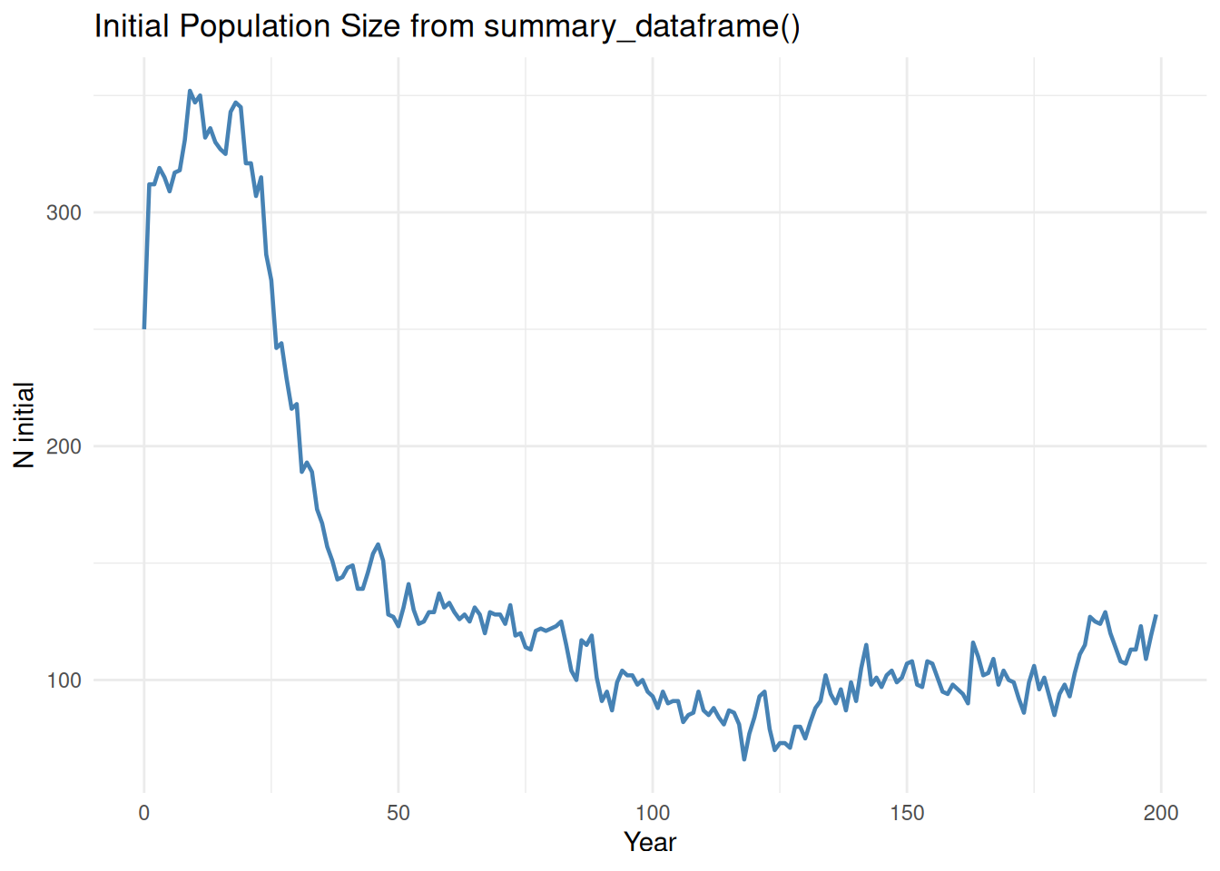
In the default long format, metrics remain in separate columns, but each pipe-delimited value is split into its own row. PatchID gives the position of the value inside the original |-delimited cell. For many summary_popAllTime columns, PatchID == 0 is the total across patches (such as N_initial) and later Patch IDs are actual patch-level values.
pop_totals <- pop_df %>%filter(PatchID ==1)ggplot(pop_totals, aes(x = Year, y = N_Initial)) +geom_line(linewidth =0.8, color ="steelblue") +labs(title ="Initial Population Size from summary_dataframe()",x ="Year",y ="N initial" ) +theme_minimal()
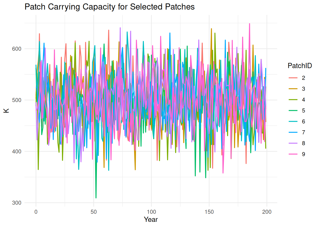
patch_subset <- pop_df %>%filter(PatchID %in%2:9)ggplot(patch_subset, aes(x = Year, y = K, color =factor(PatchID))) +geom_line(linewidth =0.7) +labs(title ="Patch Carrying Capacity for Selected Patches",x ="Year",y ="K",color ="PatchID" ) +theme_minimal()
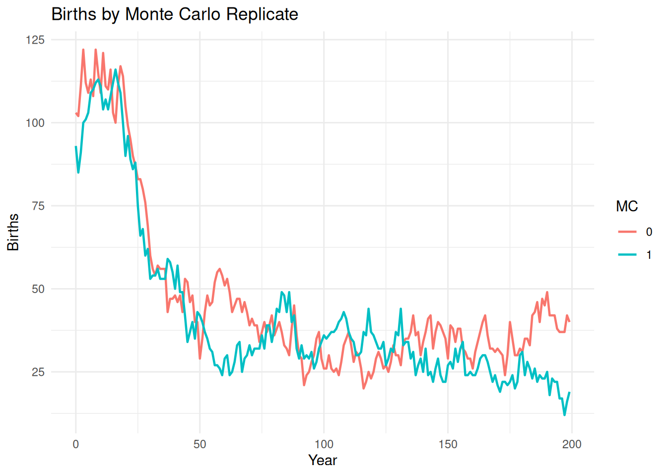
The same workflow can compare Monte Carlo replicates or batches.
pop_mc <-summary_dataframe(ex_dir, type ="pop", batch =0, mc ="all") %>%filter(PatchID ==1)ggplot(pop_mc, aes(x = Year, y = Births, color =factor(.mc), group = .mc)) +geom_line(linewidth =0.8) +labs(title ="Births by Monte Carlo Replicate",x ="Year",y ="Births",color ="MC" ) +theme_minimal()
Use summary_format = "wide" if you need the original summary columns instead.
pop_wide_df <-summary_dataframe(ex_dir, type ="pop", batch =0, mc =0, summary_format ="wide")head(pop_wide_df[, c("Year", "GrowthRate", "N_Initial")])
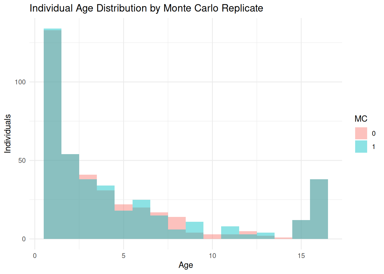
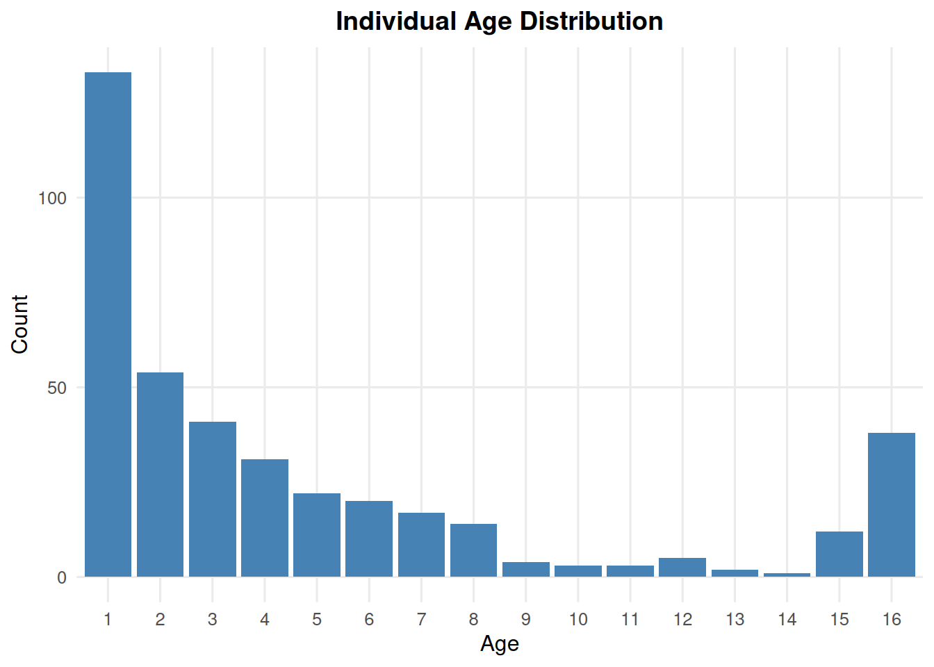
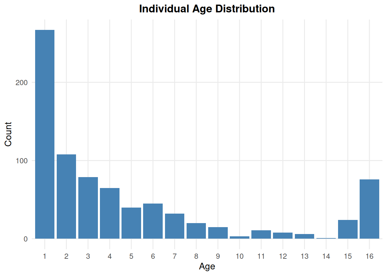
You may want to view the number of individuals in each disease state:
ind_year9 <-summary_dataframe(ex_dir, type ="ind", years =9, mc ="all")ggplot(ind_year9, aes(x = age, fill =factor(.mc))) +geom_histogram(binwidth =1, position ="identity", alpha =0.45) +labs(title ="Individual Age Distribution by Monte Carlo Replicate",x ="Age",y ="Individuals",fill ="MC" ) +theme_minimal()
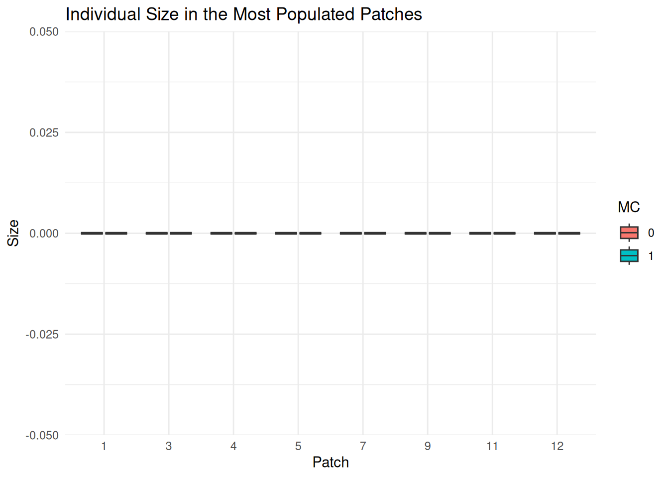
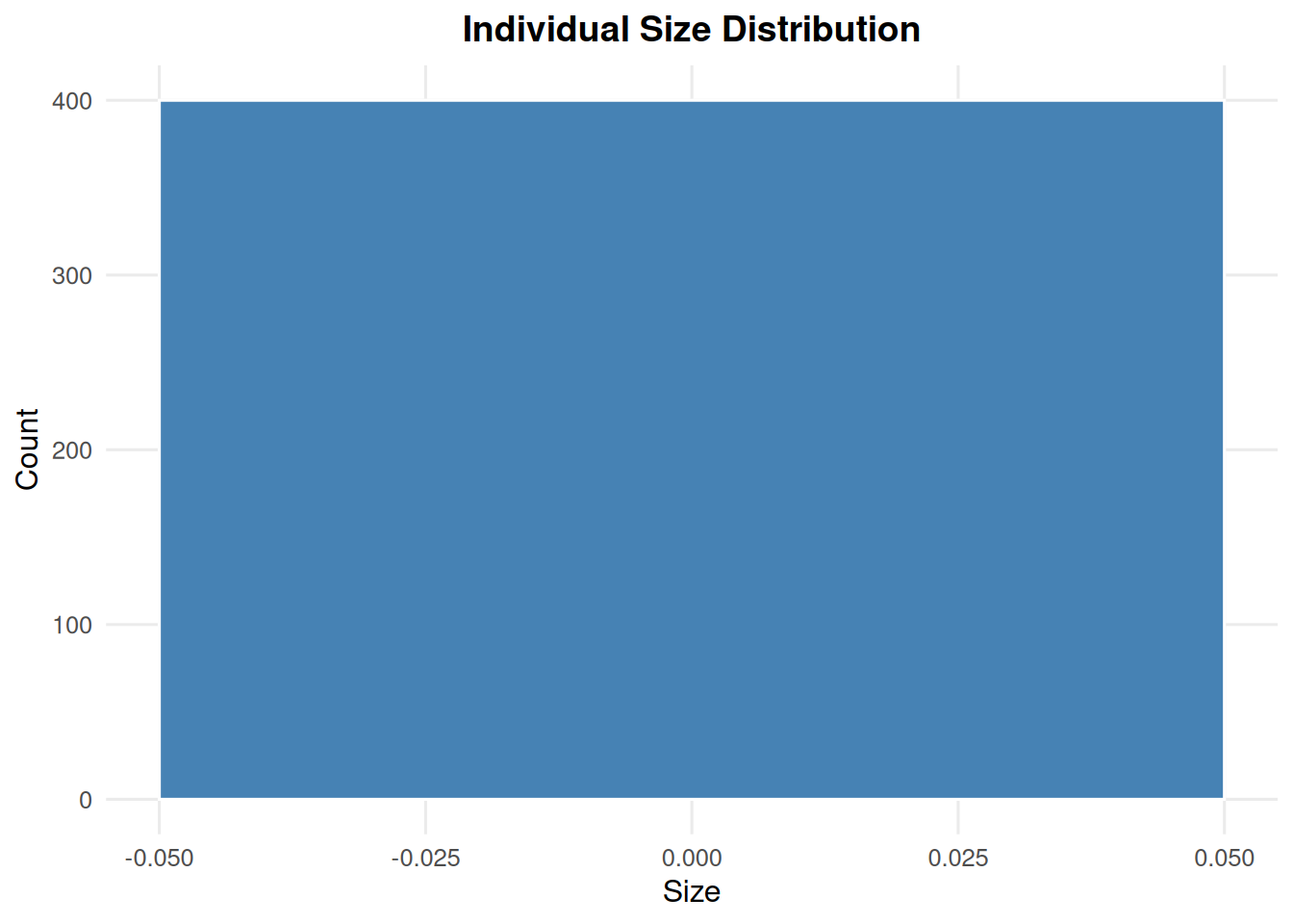
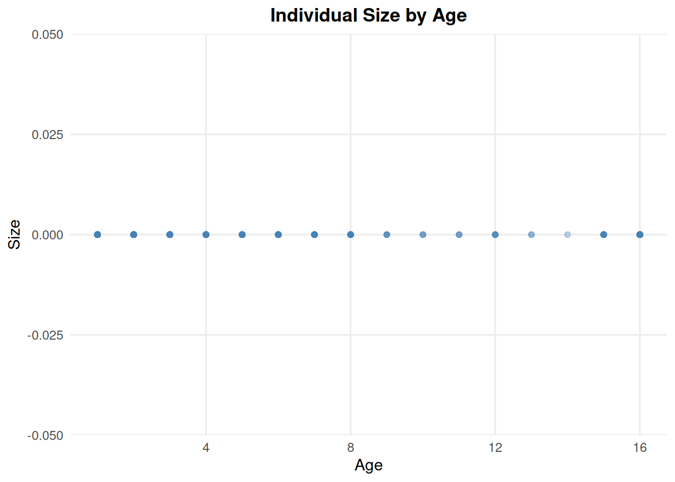
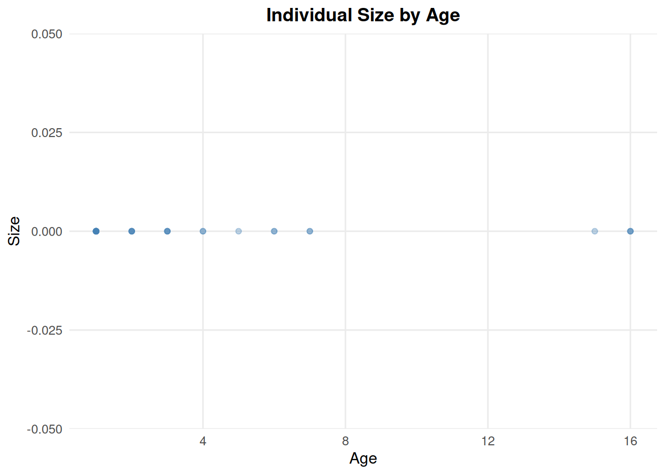
You may also examine sizes of individuals, however this does not vary in our example files:
top_patches <- ind_year9 %>%count(PatchID, sort =TRUE) %>%slice_head(n =8) %>%pull(PatchID)ind_top_patches <- ind_year9 %>%filter(PatchID %in% top_patches)ggplot(ind_top_patches, aes(x =factor(PatchID), y = size, fill =factor(.mc))) +geom_boxplot(outlier.alpha =0.3) +labs(title ="Individual Size in the Most Populated Patches",x ="Patch",y ="Size",fill ="MC" ) +theme_minimal()
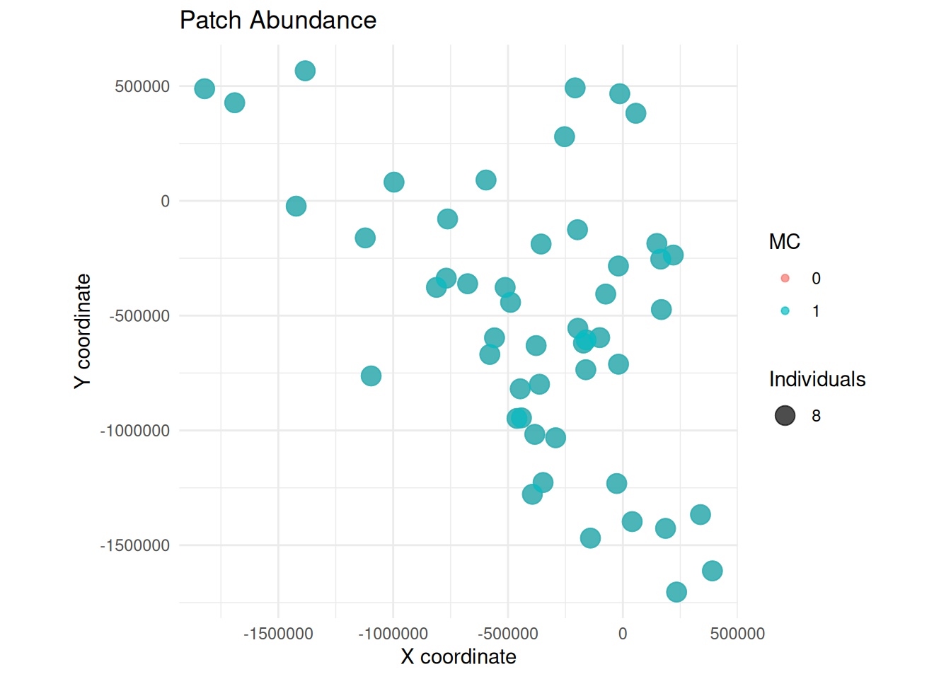
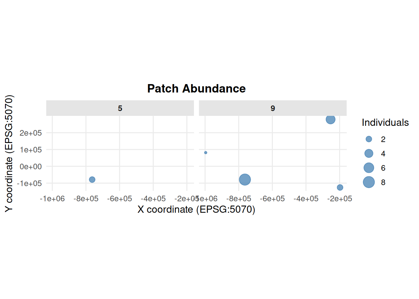
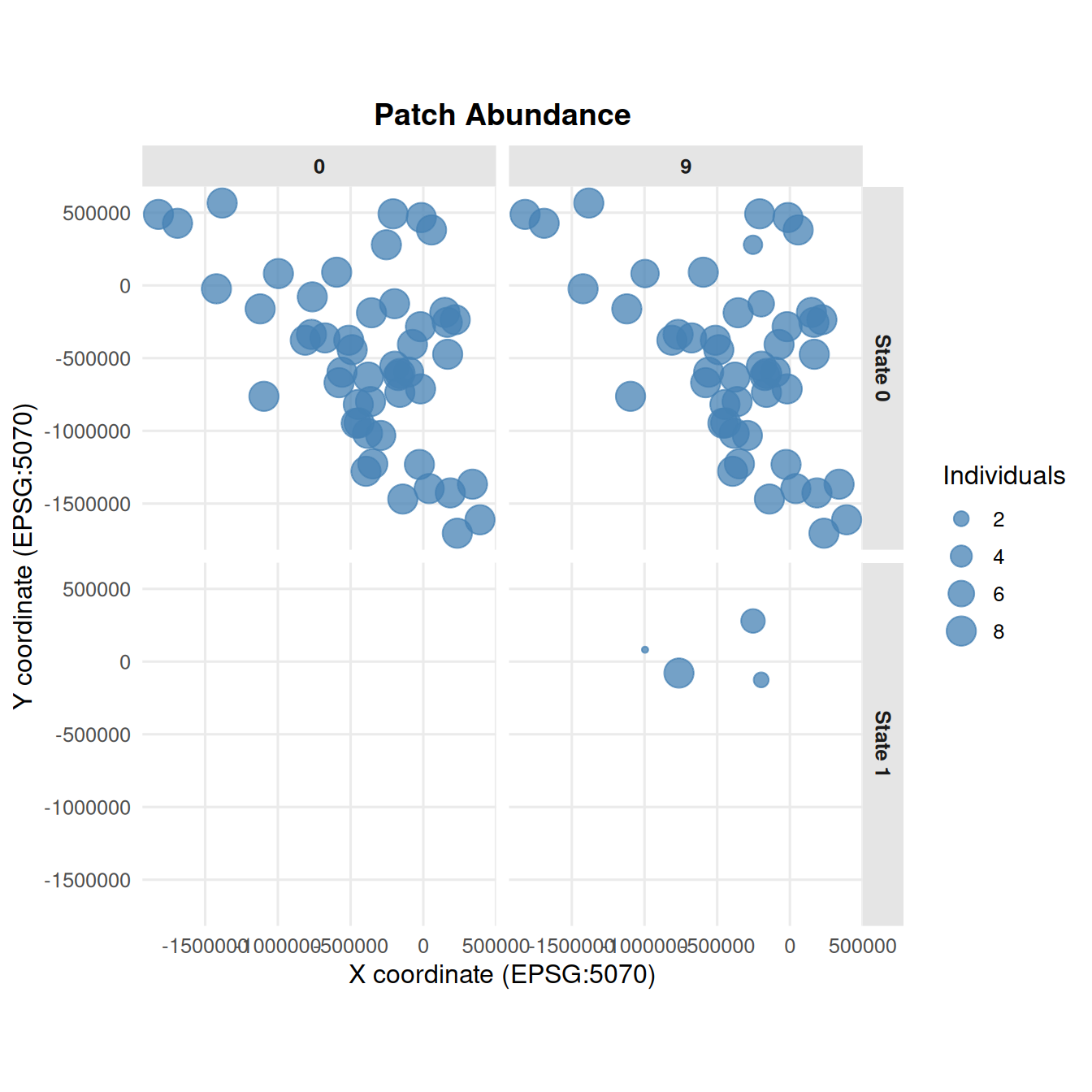
Perhaps view the distribution of individuals spatially:
If users prefer to view figures that can be made directly from CDMetaPOP outputs, they can use the following summary_pop() functions.
summary_pop() works with summary_popAllTime.csv files. The input can be a single file, a vector of files, a data frame, or a directory containing CDMetaPOP output folders.
When a directory is supplied, summary_pop() discovers the matching output folders. By default it uses run = 0, batch = 0, mc = 0, and species = 0; use "all" for any of those arguments to include multiple runs, batches, Monte Carlo replicates, or species.
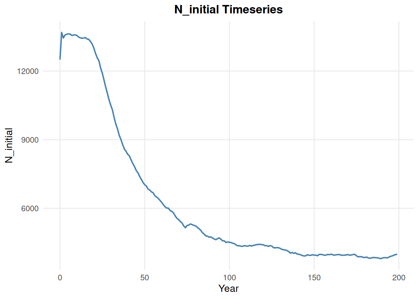
4.1 Initial Population Size
summary_pop(ex_dir, type ="N_initial")
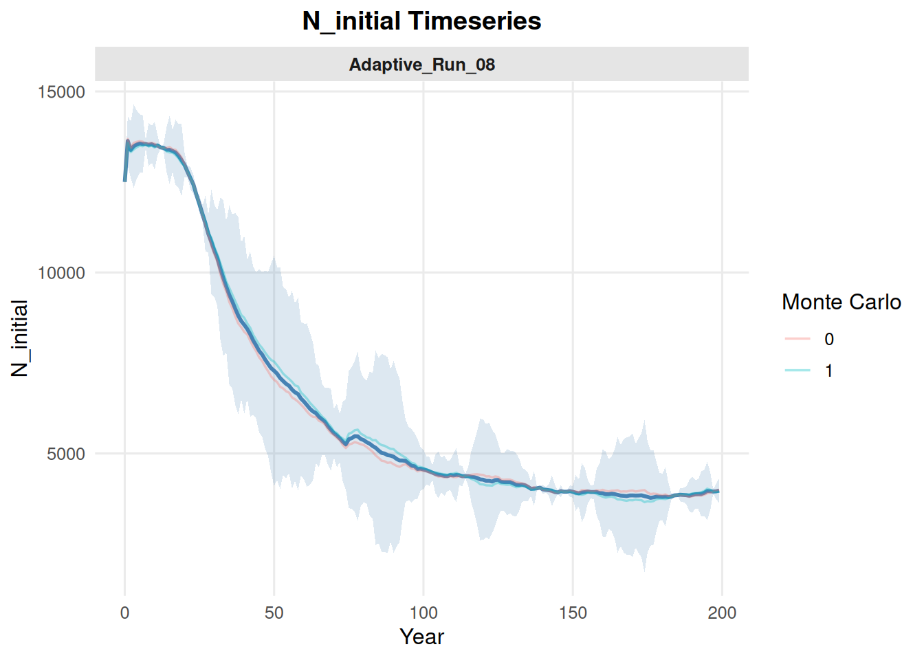
Include multiple Monte Carlo replicates by setting mc = "all". With multiple source files, the default behavior can show individual MC trajectories and a summary band.
summary_pop(ex_dir, type ="N_initial", mc ="all")
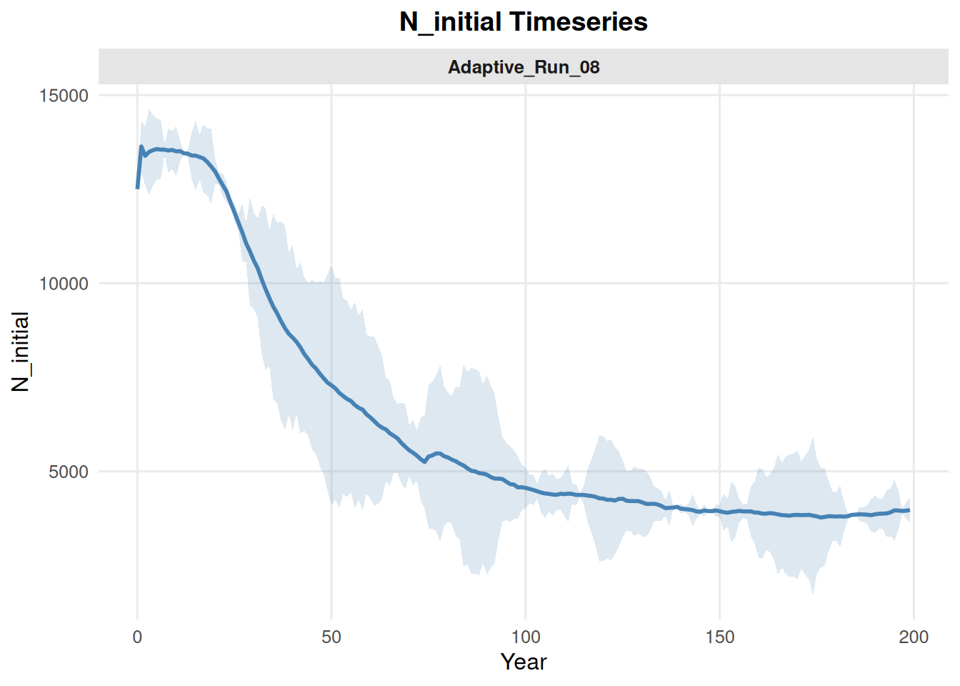
To show only the summarized pattern, set show_mc = FALSE.
summary_pop(ex_dir, type ="N_initial", mc ="all", show_mc =FALSE)
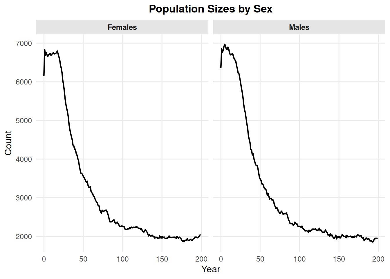
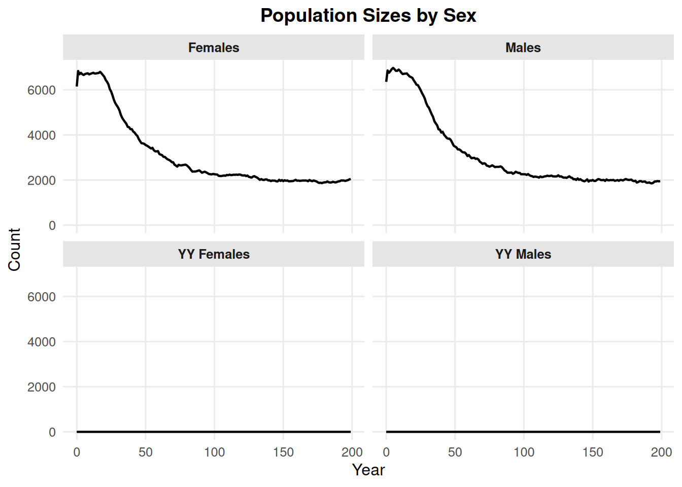
4.2 Sex Counts
By default, type = "sex" shows males and females only.
summary_pop(ex_dir, type ="sex")
Use include_yys = TRUE to include YY males and YY females. This may be relevant for fisheries research.
summary_pop(ex_dir, type ="sex", include_yys =TRUE)
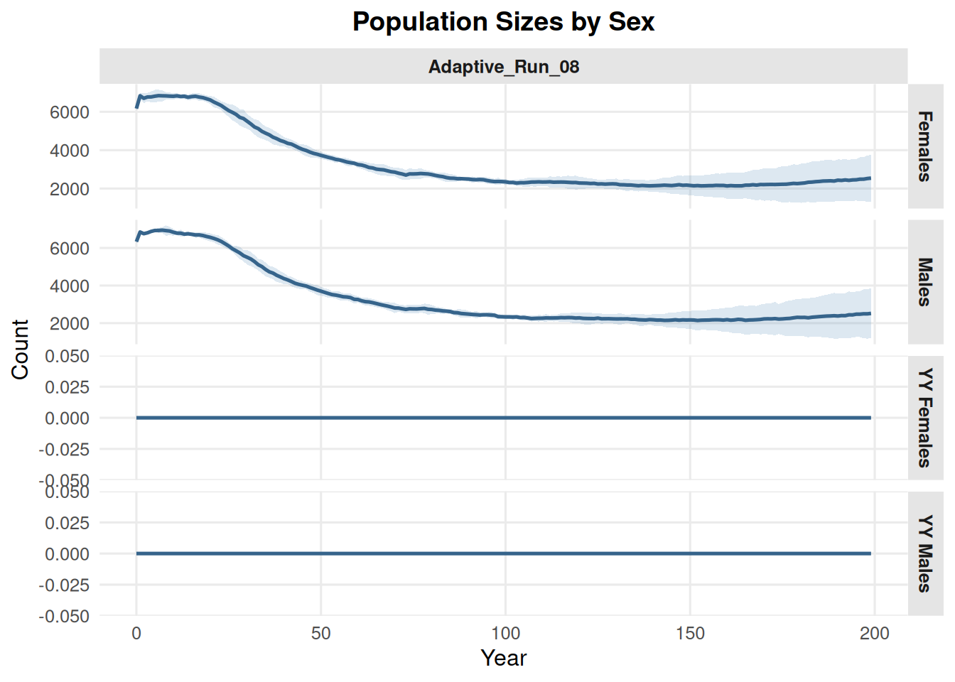
The same YY option works when comparing multiple batches or MCs.
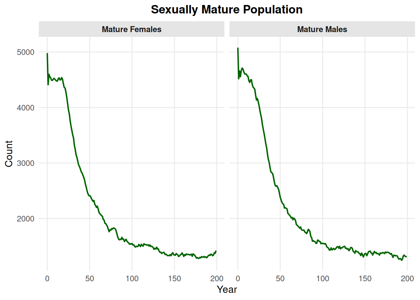
By default, type = "mature" shows mature males and mature females only.
summary_pop(ex_dir, type ="mature")
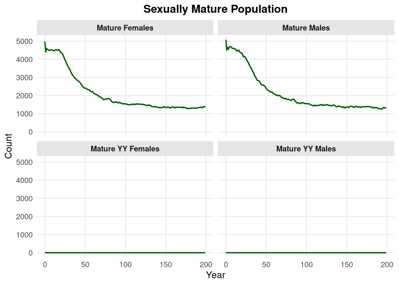
Use include_yys = TRUE to include mature YY males and mature YY females.
summary_pop(ex_dir, type ="mature", include_yys =TRUE)
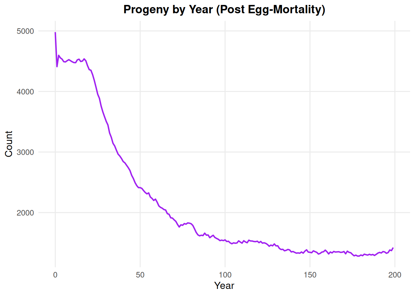
4.4 Births
summary_pop(ex_dir, type ="births")
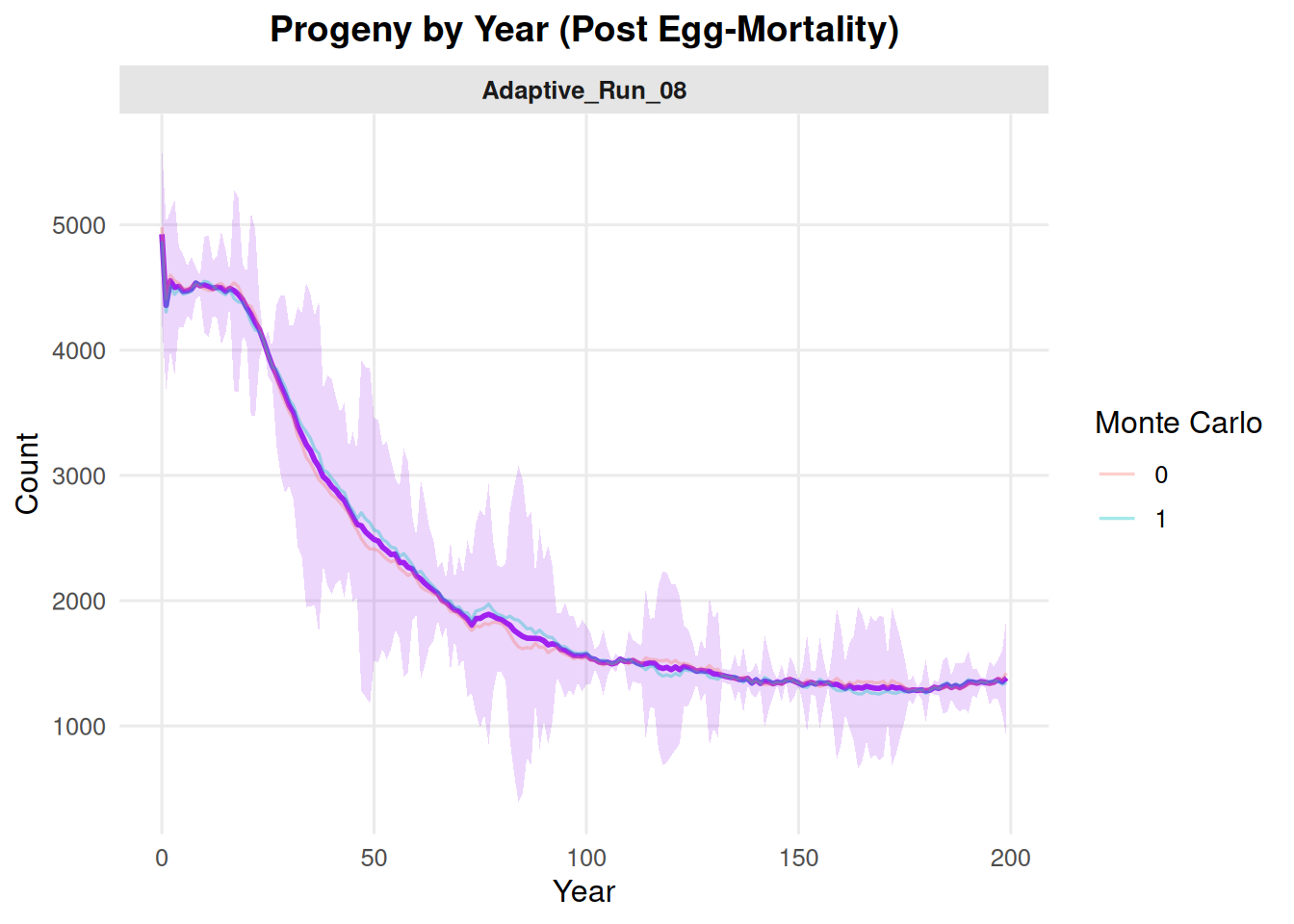
summary_pop(ex_dir, type ="births", mc ="all")
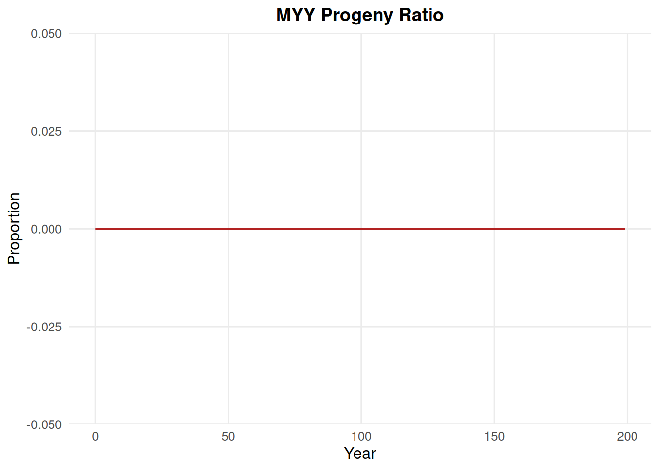
4.5 Myy Ratio
summary_pop(ex_dir, type ="myy_ratio")
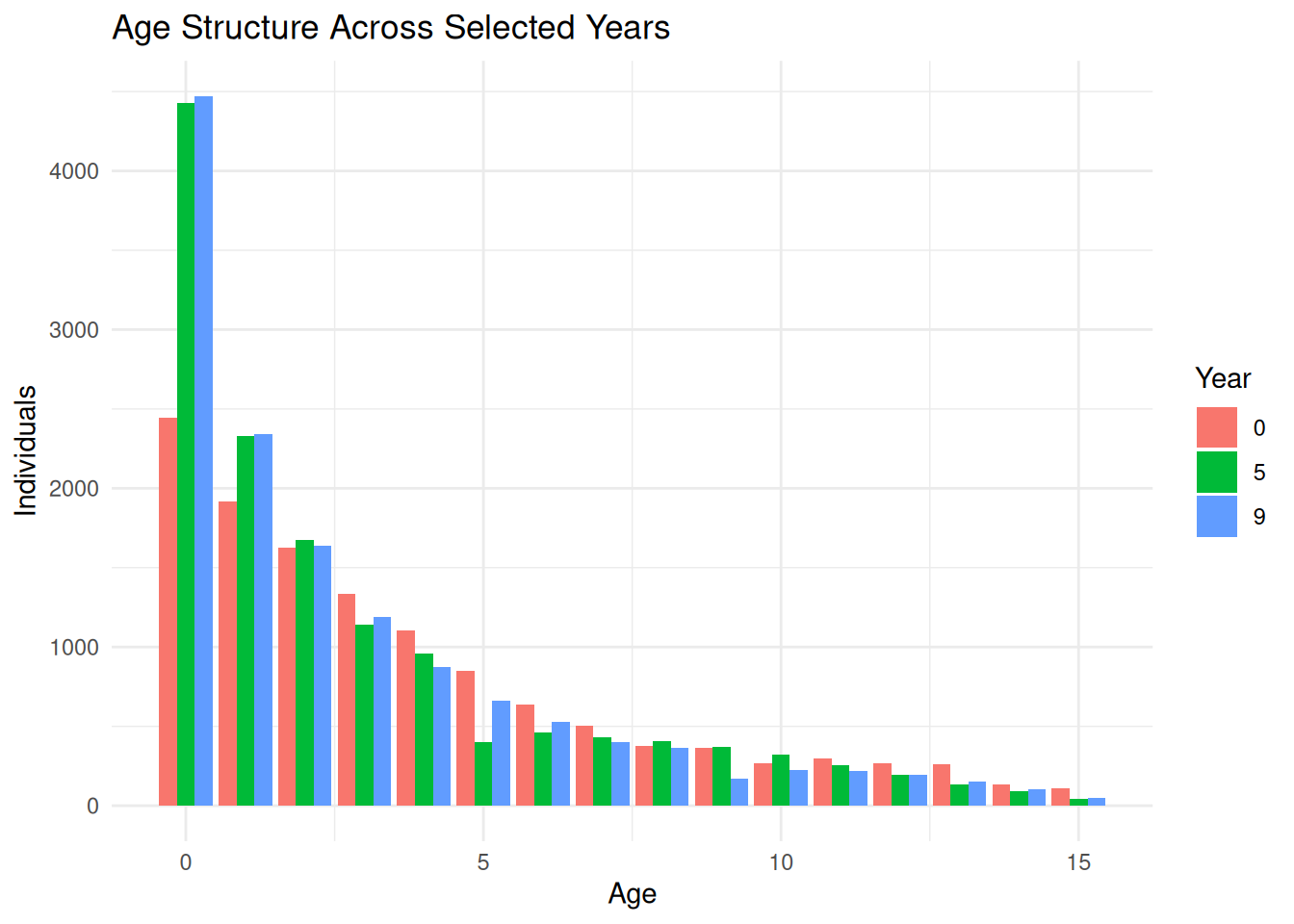
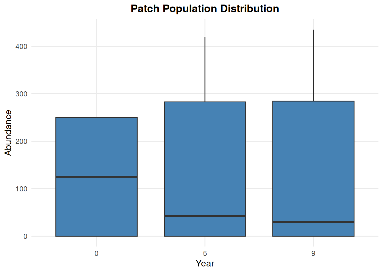
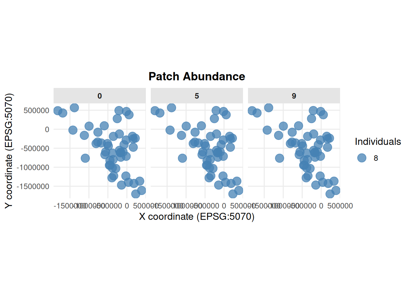
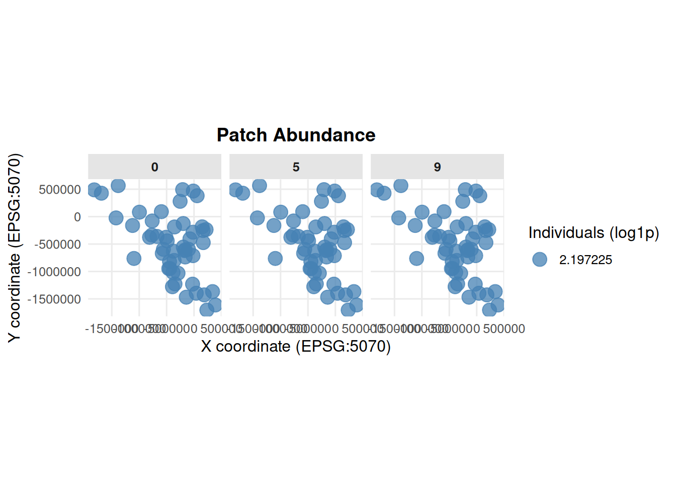
4.6 Patch Abundance from summary_popAllTime.csv
summary_pop(ex_dir, type ="patch", years =c(0, 5, 9))
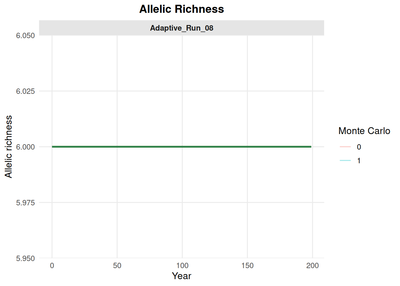
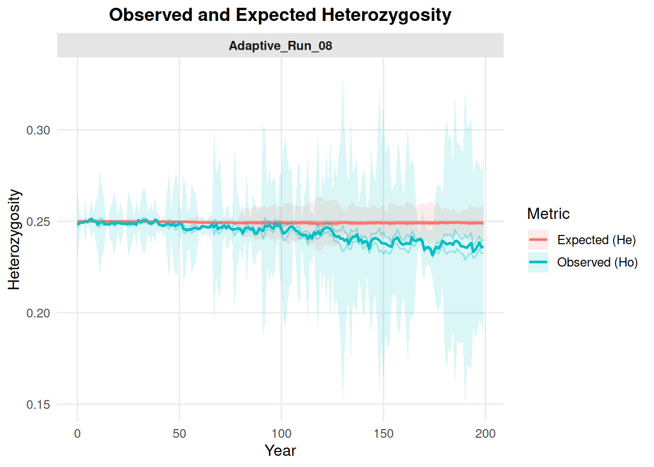
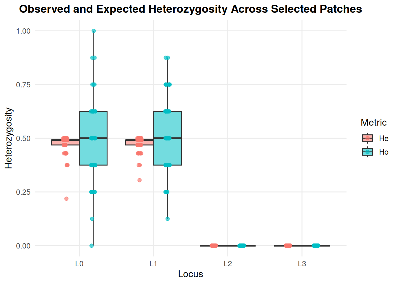
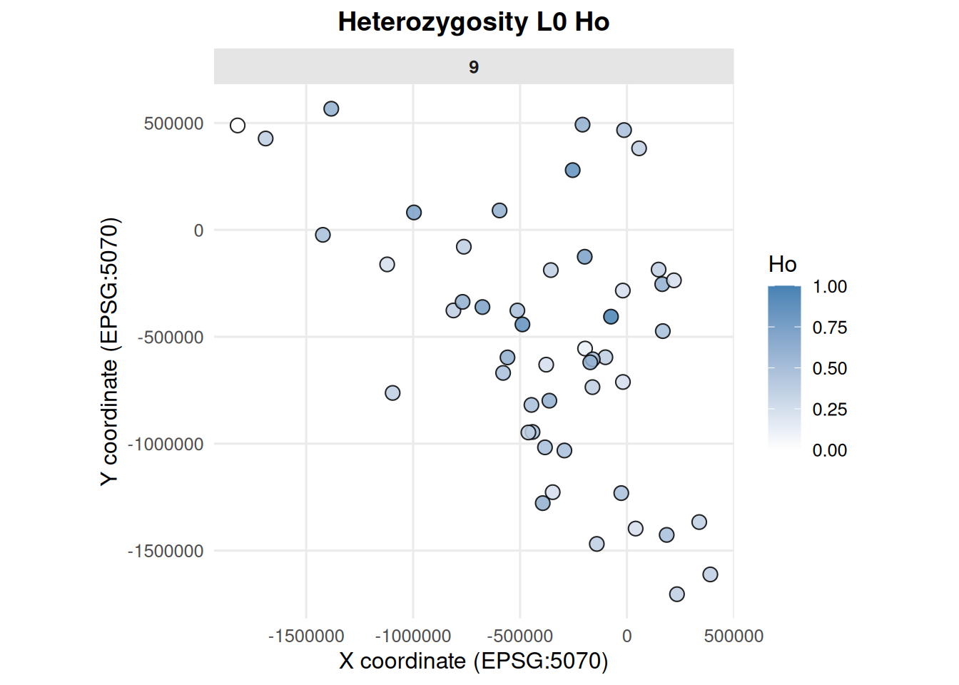
4.7 Allelic Richness and Heterozygosity from summary_popAllTime.csv
These options summarize genetic metrics stored in the population summary file.
summary_pop(ex_dir, type ="allelic_richness", mc ="all")
summary_pop(ex_dir, type ="het", mc ="all")
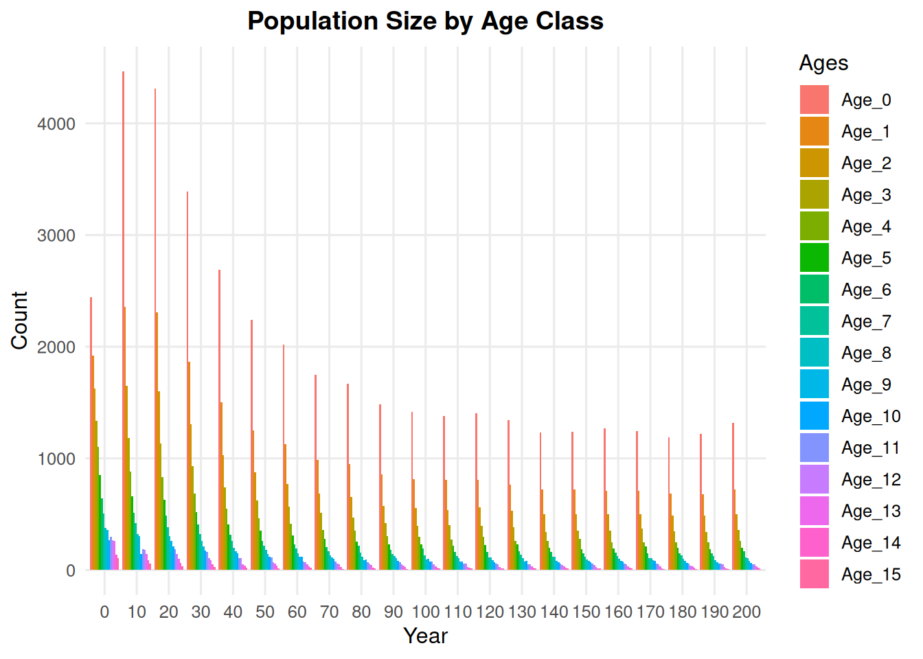
5 Class Summary Plots
summary_class() works with summary_classAllTime.csv files.
5.1 Age Class Counts
summary_class(ex_dir, type ="age_class", n =10)
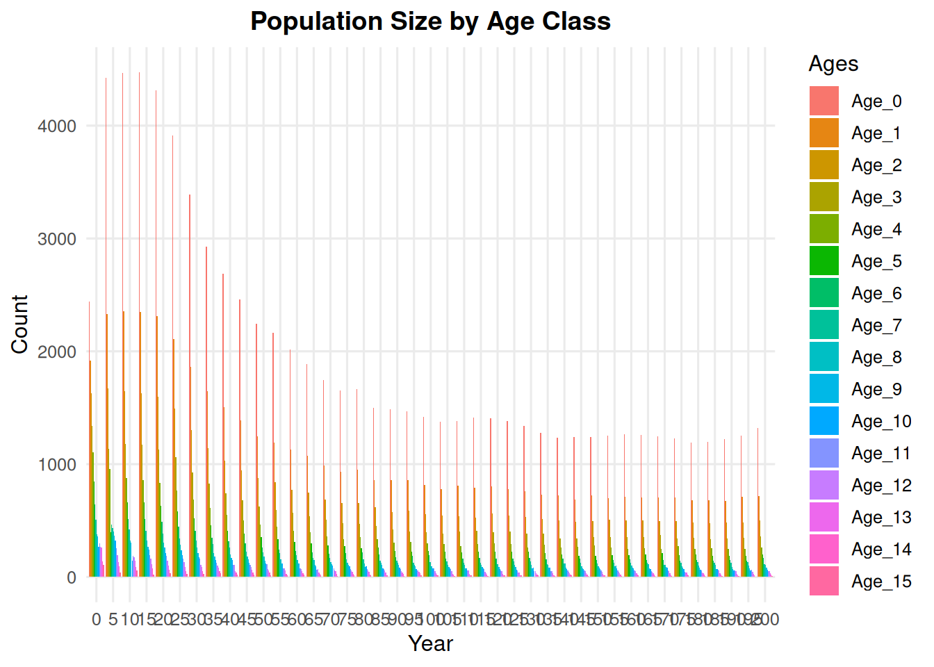
Use a smaller n to facet more years. This can be useful for short example runs or simulations with relatively few generations.
summary_class(ex_dir, type ="age_class", n =5)
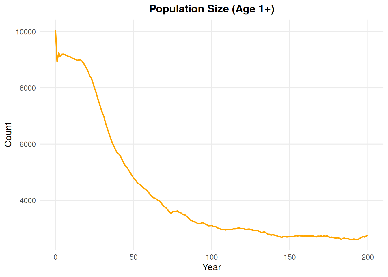
5.2 Age Plus One
summary_class(ex_dir, type ="age_plus_one")
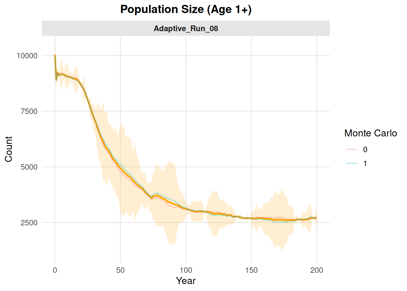
summary_class(ex_dir, type ="age_plus_one", mc ="all")
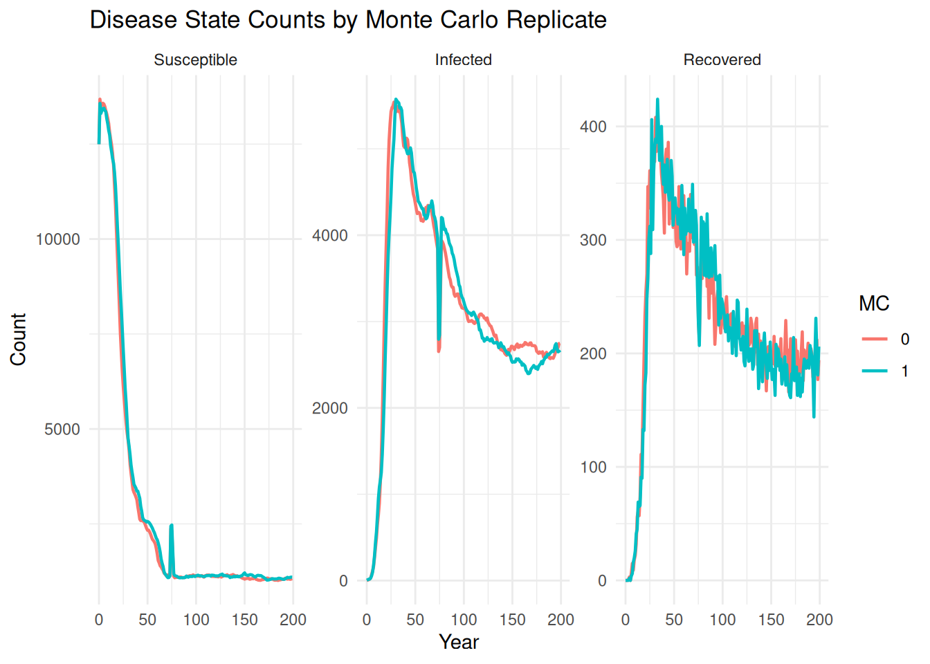
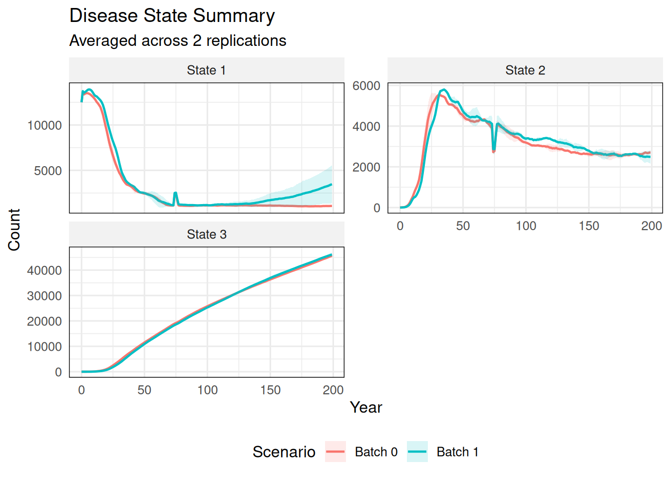
6 Disease State Summaries
summarize_states() works with summary_popAllTime_DiseaseStates.csv files. It summarizes disease-state counts across Monte Carlo replicates and compares batches.
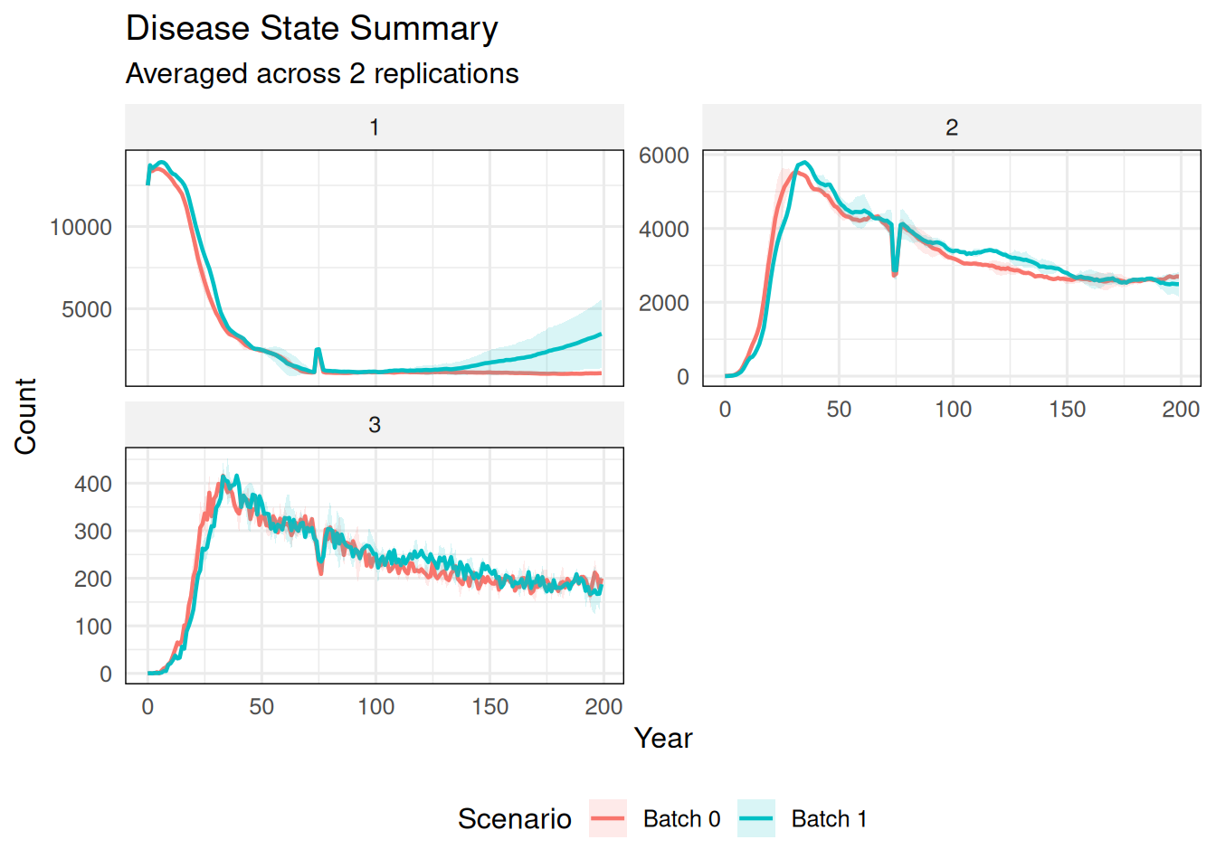
6.1 Default State Names
summarize_states(ex_dir)
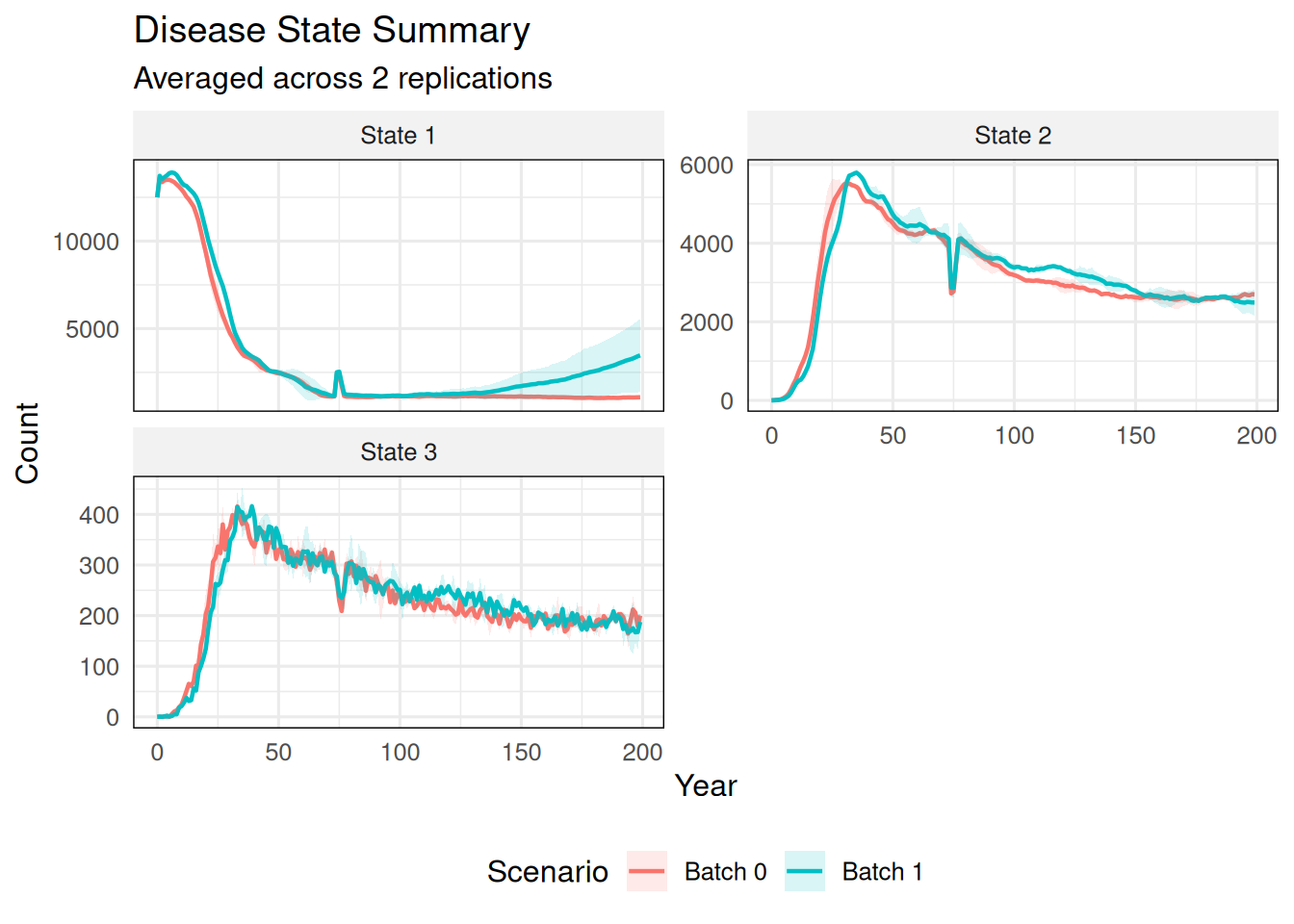
6.2 Custom State and Scenario Names
summarize_states( ex_dir,state_names =c("State 1", "State 2", "State 3"),scenario_names =c("Batch 0", "Batch 1"))
6.3 Cumulative State
Use cumulative_states for a state that should be plotted as a running total within each Monte Carlo replicate.
summarize_states( ex_dir,state_names =c("State 1", "State 2", "State 3"),scenario_names =c("Batch 0", "Batch 1"),cumulative_states ="State 3")
7 Individual File Summaries
summary_ind() works with ind##.csv files. The input can be one file, multiple files, a run folder, a top-level output directory, or a data frame.
For one-year plots, specify year. For movement over time, specify years.
7.1 Age Histogram
summary_ind(ex_dir, type ="age", year =9, batch =0, mc =0)
summary_ind(ex_dir, type ="age", year =9, batch =0, mc ="all")
7.2 Size Histogram
summary_ind(ex_dir, type ="size", year =9, batch =0, mc =0)
7.3 Size by Age
summary_ind(ex_dir, type ="age_size", year =9, batch =0, mc =0)
Filter to a subset of patches with patches.
summary_ind(ex_dir, type ="age_size", year =9, batch =0, mc =0, patches =c(1, 3, 4, 5))
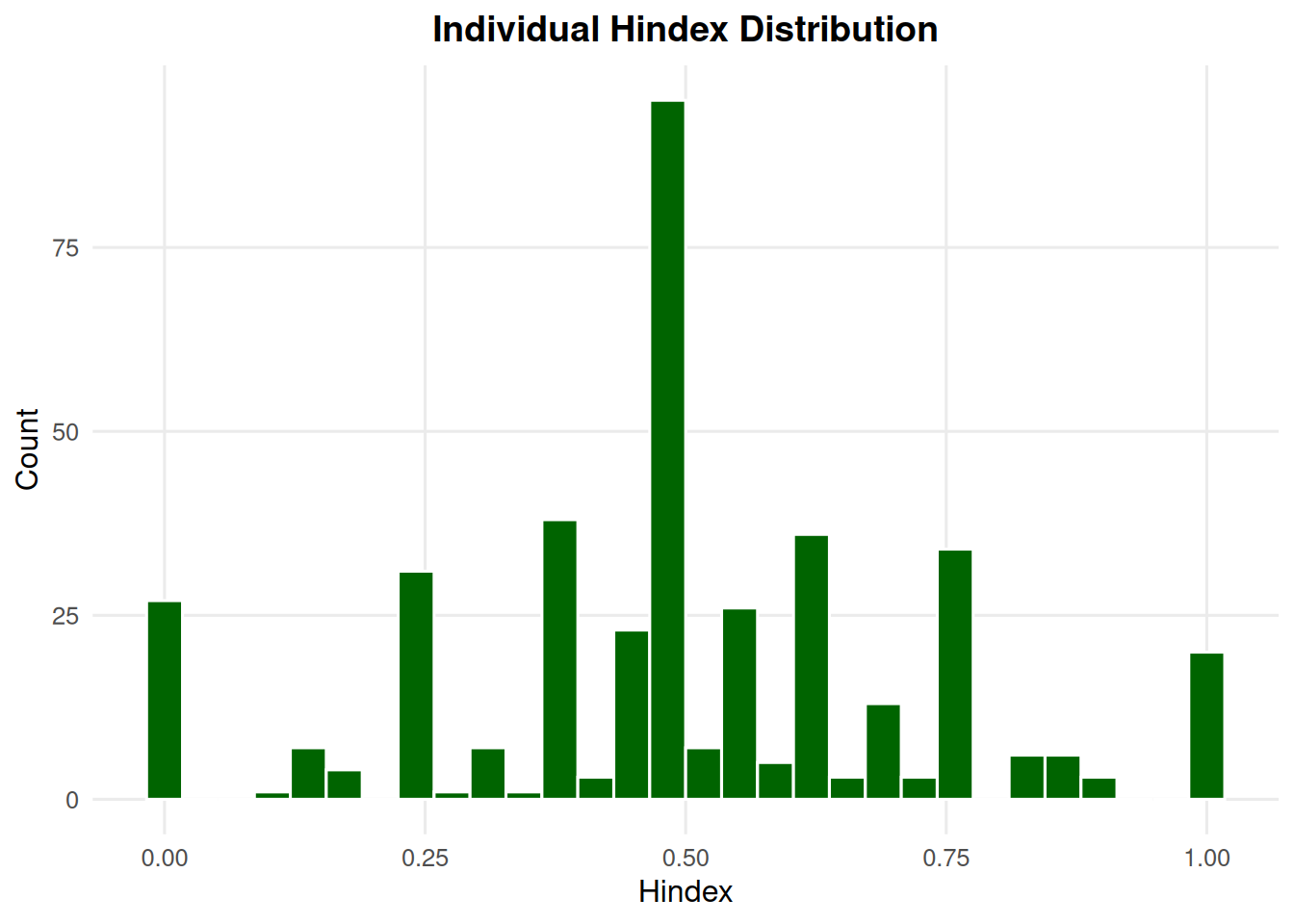
7.4 Hindex Histogram
summary_ind(ex_dir, type ="hindex", year =9, batch =0, mc =0)
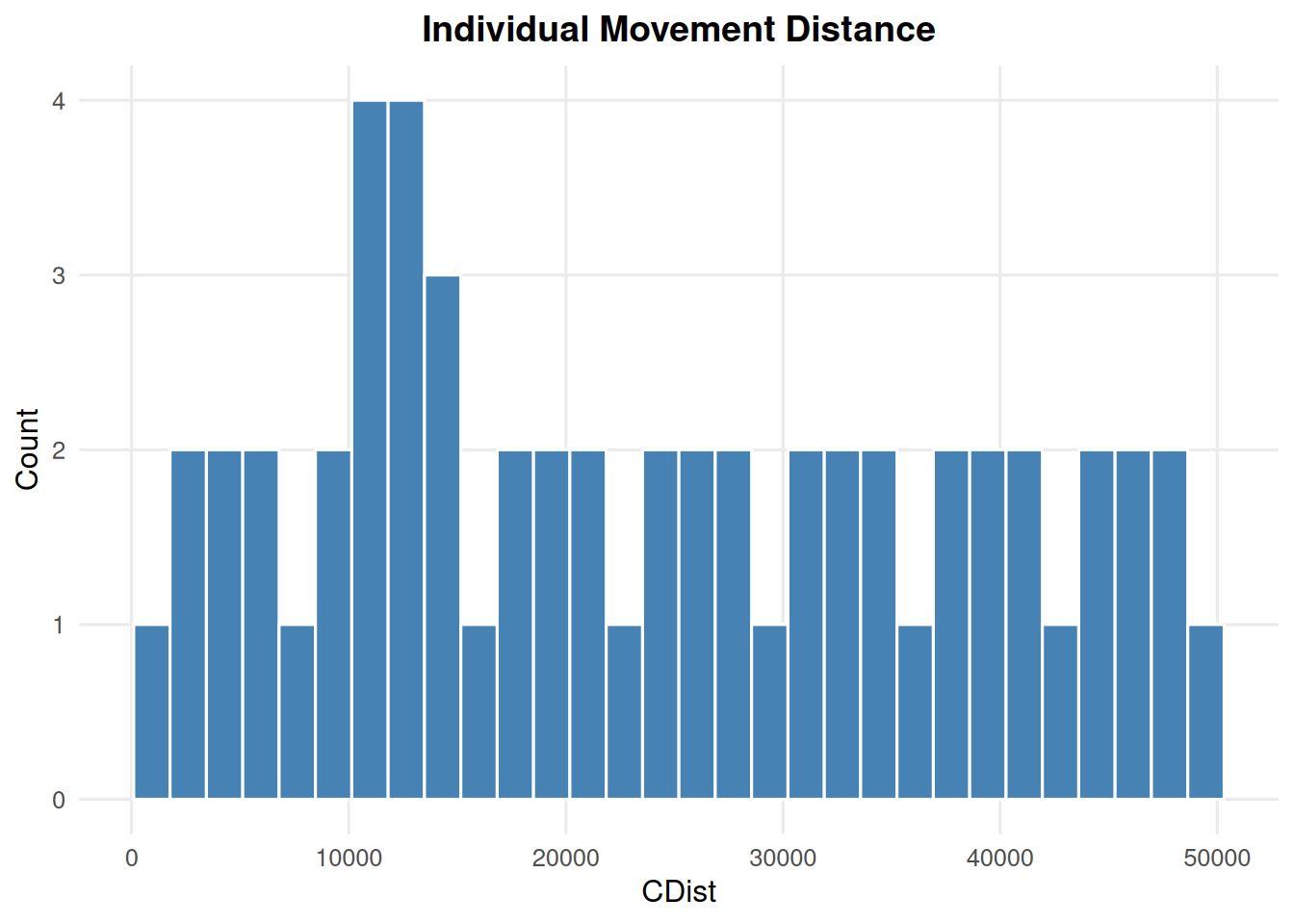
7.5 Movement Distance Histogram
CDist = -9999 is treated as no movement and is excluded from the histogram.
summary_ind(ex_dir, type ="cdist", year =9, batch =0, mc =0)
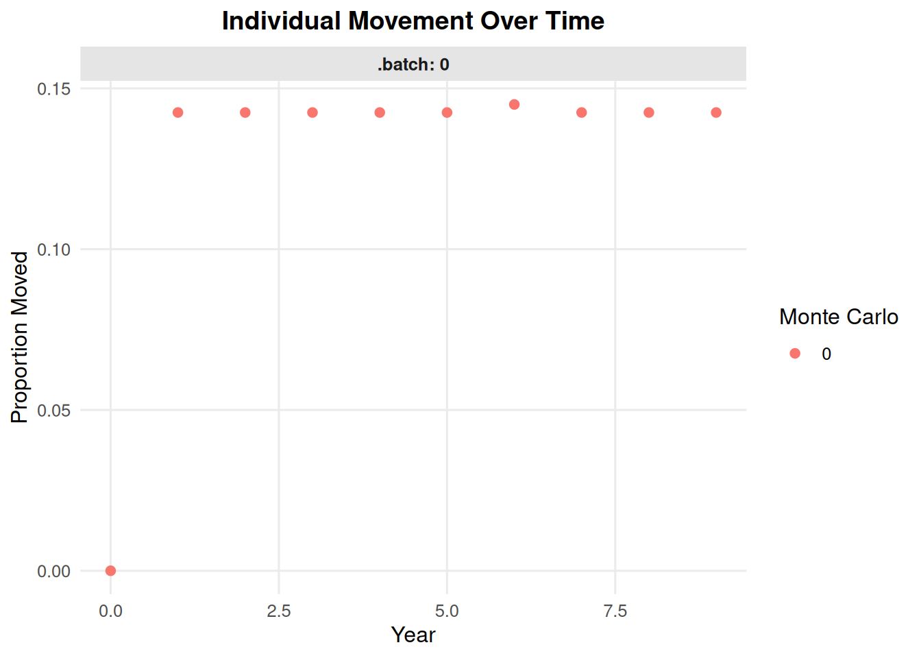
7.6 Movement Over Time
summary_ind(ex_dir, type ="movement", years =0:9, batch =0, mc =0)
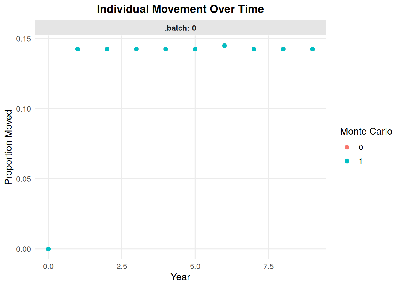
summary_ind(ex_dir, type ="movement", years =0:9, batch =0, mc ="all")
If CDMetaPOP output includes sampled individual files, use file_type = "ind_Sample" to read ind##_Sample.csv files instead of ind##.csv files. The bundled example data use ind##.csv, so this example is shown but not evaluated.
summary_ind(ex_dir, type ="age", year =9, file_type ="ind_Sample")
8 Individual-Level Genetics
The individual-level genetics functions use genotype columns named like L0A0, L0A1, L1A0, and so on.
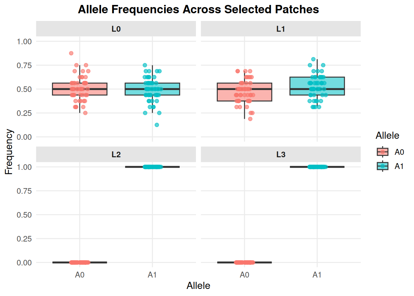
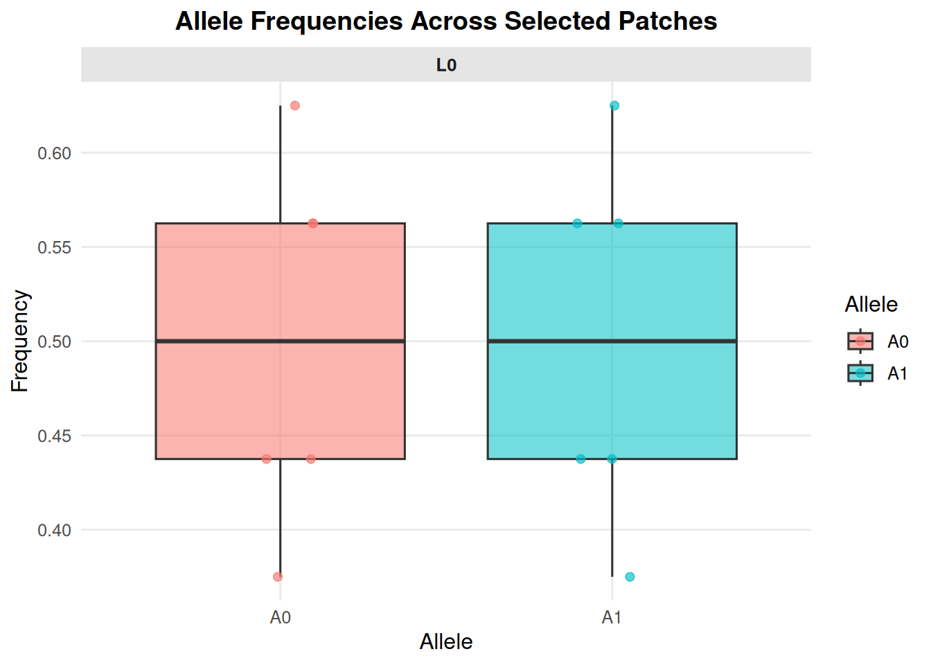
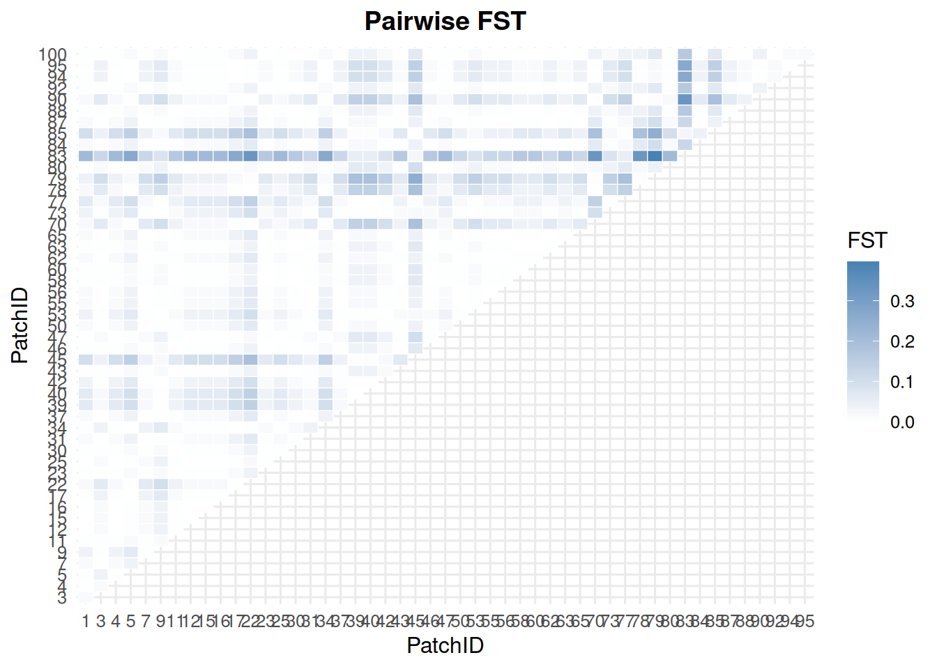
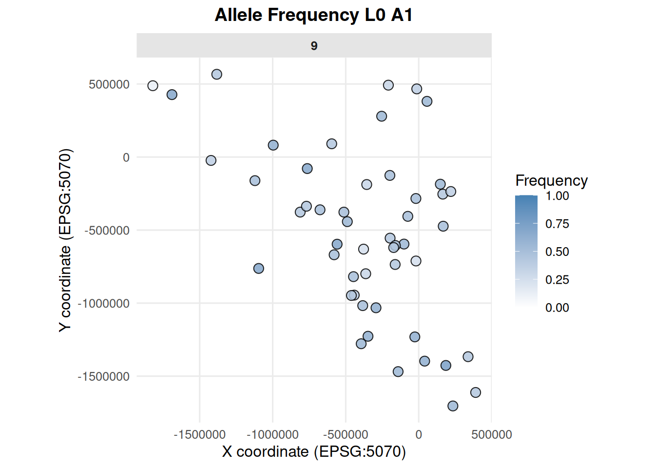
8.1 Allele Frequencies by Patch
allele_frequencies_ind(ex_dir, year =9, batch =0, mc =0)
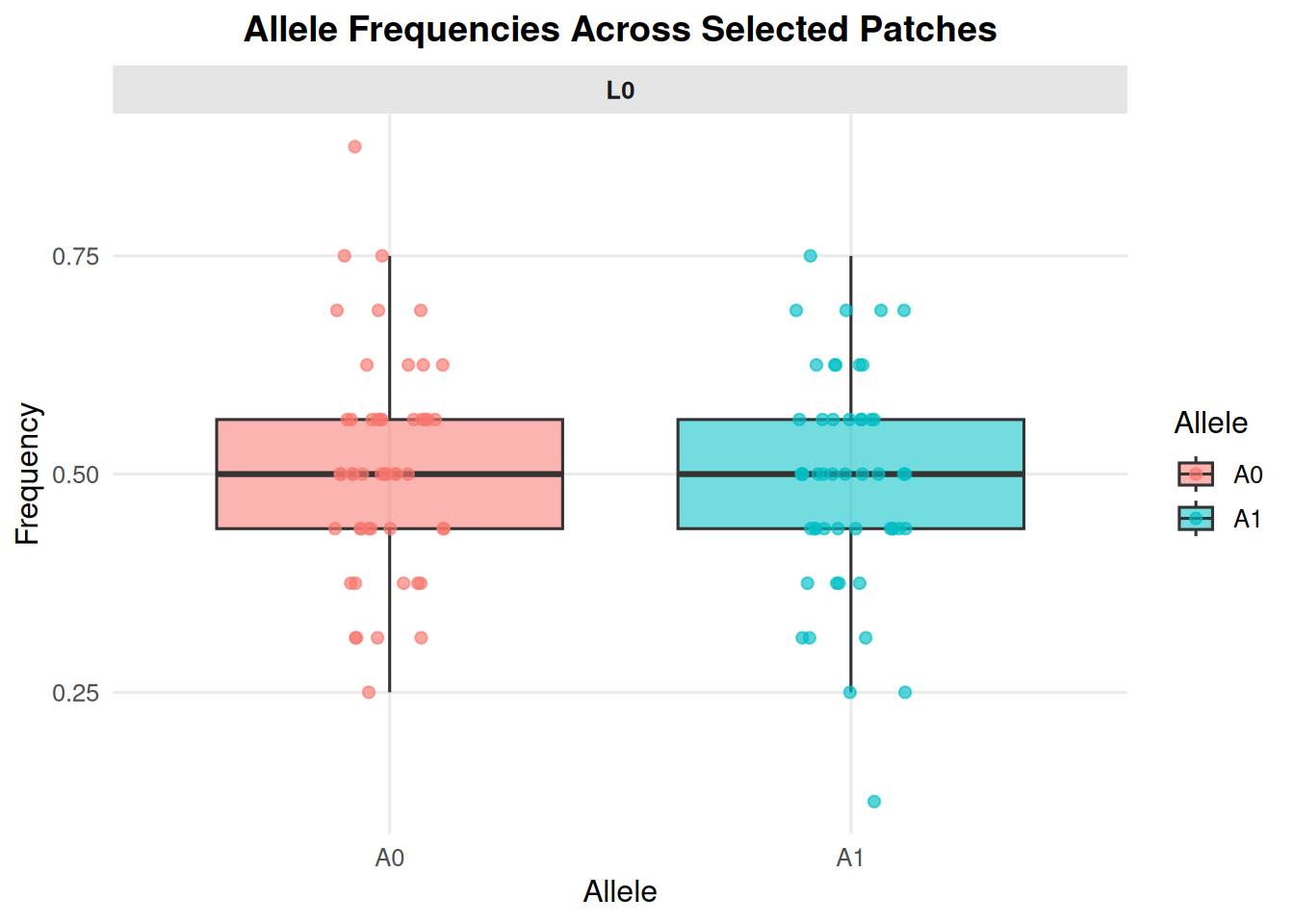
Focus on one locus with loci.
allele_frequencies_ind(ex_dir, year =9, batch =0, mc =0, loci ="L0")
Filter to selected patches when a figure would otherwise be too dense.
The following functions are exported, but they launch external software or interactive Shiny apps. They are shown here as code examples but are not run while knitting this document.
locus() is exported for compatibility with older gstudio workflows. It is included in the package because the original function is deprecated elsewhere.